Generating Random Sentence with LSTM RNN
This tutorial shows how to train a LSTM (Long short-term memory) RNN (recurrent
neural network) to perform character-level sequence training and prediction. The
original model, usually called char-rnn is described in Andrej Karpathy’s
blog, with
a reference implementation in Torch available here.
Because MXNet.jl does not have a specialized model for recurrent neural networks
yet, the example shown here is an implementation of LSTM by using the default
FeedForward model via explicitly unfolding over time. We will be using
fixed-length input sequence for training. The code is adapted from the char-rnn
example for MXNet’s Python binding, which
demonstrates how to use low-level symbolic APIs to
build customized neural network models directly.
The most important code snippets of this example is shown and explained here. To see and run the complete code, please refer to the examples/char-lstm directory. You will need to install Iterators.jl and StatsBase.jl to run this example.
LSTM Cells
Christopher Olah has a great blog post about LSTM with beautiful and
clear illustrations. So we will not repeat the definition and explanation of
what an LSTM cell is here. Basically, an LSTM cell takes input x, as well as
previous states (including c and h), and produce the next states.
We define a helper type to bundle the two state variables together:
immutable LSTMState
  c :: mx.SymbolicNode
  h :: mx.SymbolicNode
end
Because LSTM weights are shared at every time when we do explicit unfolding, so we also define a helper type to hold all the weights (and bias) for an LSTM cell for convenience.
immutable LSTMParam
  i2h_W :: mx.SymbolicNode
  h2h_W :: mx.SymbolicNode
  i2h_b :: mx.SymbolicNode
  h2h_b :: mx.SymbolicNode
end
Note all the variables are of type SymbolicNode. We will construct the
LSTM network as a symbolic computation graph, which is then instantiated with
NDArray for actual computation.
function lstm_cell(data::mx.SymbolicNode, prev_state::LSTMState, param::LSTMParam;
                   num_hidden::Int=512, dropout::Real=0, name::Symbol=gensym())

  if dropout > 0
    data = mx.Dropout(data, p=dropout)
  end

  i2h = mx.FullyConnected(data=data, weight=param.i2h_W, bias=param.i2h_b,
                          num_hidden=4num_hidden, name=symbol(name, "_i2h"))
  h2h = mx.FullyConnected(data=prev_state.h, weight=param.h2h_W, bias=param.h2h_b,
                          num_hidden=4num_hidden, name=symbol(name, "_h2h"))

  gates = mx.SliceChannel(i2h + h2h, num_outputs=4, name=symbol(name, "_gates"))

  in_gate     = mx.Activation(gates[1], act_type=:sigmoid)
  in_trans    = mx.Activation(gates[2], act_type=:tanh)
  forget_gate = mx.Activation(gates[3], act_type=:sigmoid)
  out_gate    = mx.Activation(gates[4], act_type=:sigmoid)

  next_c = (forget_gate .* prev_state.c) + (in_gate .* in_trans)
  next_h = out_gate .* mx.Activation(next_c, act_type=:tanh)

  return LSTMState(next_c, next_h)
end
The following figure is stolen (permission requested) from Christopher Olah’s blog, which illustrate exactly what the code snippet above is doing.
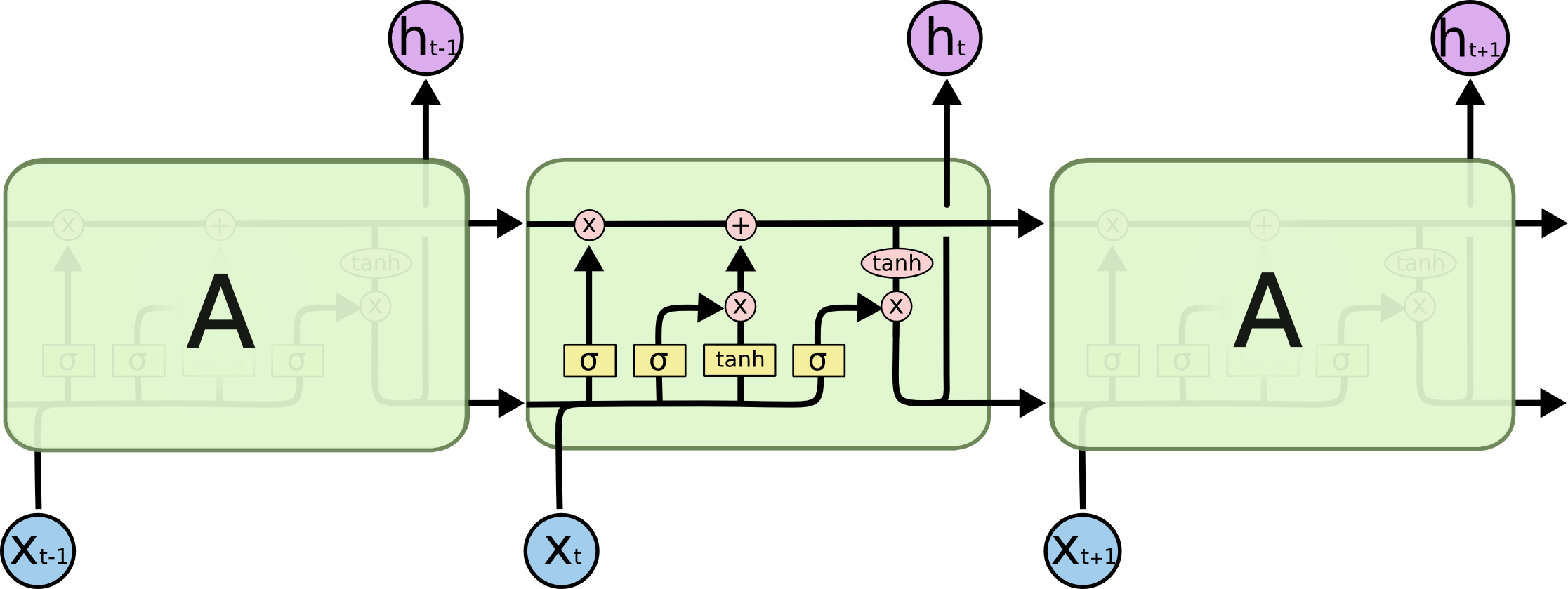
In particular, instead of defining the four gates independently, we do the
computation together and then use SliceChannel to split them into four
outputs. The computation of gates are all done with the symbolic API. The return
value is a LSTM state containing the output of a LSTM cell.
Unfolding LSTM
Using the LSTM cell defined above, we are now ready to define a function to unfold a LSTM network with L layers and T time steps. The first part of the function is just defining all the symbolic variables for the shared weights and states.
The embed_W is the weights used for character embedding — i.e. mapping the
one-hot encoded characters into real vectors. The pred_W and pred_b are
weights and bias for the final prediction at each time step.
Then we define the weights for each LSTM cell. Note there is one cell for each layer, and it will be replicated (unrolled) over time. The states are, however, not shared over time. Instead, here we define the initial states here at the beginning of a sequence, and we will update them with the output states at each time step as we explicitly unroll the LSTM.
function LSTM(n_layer::Int, seq_len::Int, dim_hidden::Int, dim_embed::Int, n_class::Int;
              dropout::Real=0, name::Symbol=gensym(), output_states::Bool=false)

  # placeholder nodes for all parameters
  embed_W = mx.Variable(symbol(name, "_embed_weight"))
  pred_W  = mx.Variable(symbol(name, "_pred_weight"))
  pred_b  = mx.Variable(symbol(name, "_pred_bias"))

  layer_param_states = map(1:n_layer) do i
    param = LSTMParam(mx.Variable(symbol(name, "_l$(i)_i2h_weight")),
                      mx.Variable(symbol(name, "_l$(i)_h2h_weight")),
                      mx.Variable(symbol(name, "_l$(i)_i2h_bias")),
                      mx.Variable(symbol(name, "_l$(i)_h2h_bias")))
    state = LSTMState(mx.Variable(symbol(name, "_l$(i)_init_c")),
                      mx.Variable(symbol(name, "_l$(i)_init_h")))
    (param, state)
  end
  #...
Unrolling over time is a straightforward procedure of stacking the embedding
layer, and then LSTM cells, on top of which the prediction layer. During
unrolling, we update the states and collect all the outputs. Note each time step
takes data and label as inputs. If the LSTM is named as :ptb, the data and
label at step t will be named :ptb_data_$t and :ptb_label_$t. Late
on when we prepare the data, we will define the data provider to match those
names.
  # now unroll over time
  outputs = mx.SymbolicNode[]
  for t = 1:seq_len
    data   = mx.Variable(symbol(name, "_data_$t"))
    label  = mx.Variable(symbol(name, "_label_$t"))
    hidden = mx.FullyConnected(data=data, weight=embed_W, num_hidden=dim_embed,
                               no_bias=true, name=symbol(name, "_embed_$t"))

    # stack LSTM cells
    for i = 1:n_layer
      l_param, l_state = layer_param_states[i]
      dp = i == 1 ? 0 : dropout # don't do dropout for data
      next_state = lstm_cell(hidden, l_state, l_param, num_hidden=dim_hidden, dropout=dp,
                             name=symbol(name, "_lstm_$t"))
      hidden = next_state.h
      layer_param_states[i] = (l_param, next_state)
    end

    # prediction / decoder
    if dropout > 0
      hidden = mx.Dropout(hidden, p=dropout)
    end
    pred = mx.FullyConnected(data=hidden, weight=pred_W, bias=pred_b, num_hidden=n_class,
                             name=symbol(name, "_pred_$t"))
    smax = mx.SoftmaxOutput(pred, label, name=symbol(name, "_softmax_$t"))
    push!(outputs, smax)
  end
  #...
Note at each time step, the prediction is connected to a SoftmaxOutput
operator, which could back propagate when corresponding labels are provided. The
states are then connected to the next time step, which allows back propagate
through time. However, at the end of the sequence, the final states are not
connected to anything. This dangling outputs is problematic, so we explicitly
connect each of them to a BlockGrad operator, which simply back
propagates 0-gradient and closes the computation graph.
In the end, we just group all the prediction outputs at each time step as
a single SymbolicNode and return. Optionally we will also group the
final states, this is used when we use the trained LSTM to sample sentences.
  # append block-gradient nodes to the final states
  for i = 1:n_layer
    l_param, l_state = layer_param_states[i]
    final_state = LSTMState(mx.BlockGrad(l_state.c, name=symbol(name, "_l$(i)_last_c")),
                            mx.BlockGrad(l_state.h, name=symbol(name, "_l$(i)_last_h")))
    layer_param_states[i] = (l_param, final_state)
  end

  # now group all outputs together
  if output_states
    outputs = outputs ∪ [x[2].c for x in layer_param_states] ∪
                        [x[2].h for x in layer_param_states]
  end
  return mx.Group(outputs...)
end
Data Provider for Text Sequences
Now we need to construct a data provider that takes a text file, divide the text into mini-batches of fixed-length character-sequences, and provide them as one-hot encoded vectors.
Note the is no fancy feature extraction at all. Each character is simply encoded as a one-hot vector: a 0-1 vector of the size given by the vocabulary. Here we just construct the vocabulary by collecting all the unique characters in the training text – there are not too many of them (including punctuations and whitespace) for English text. Each input character is then encoded as a vector of 0s on all coordinates, and 1 on the coordinate corresponding to that character. The character-to-coordinate mapping is giving by the vocabulary.
The text sequence data provider implement the data provider API. We define the CharSeqProvider as below:
type CharSeqProvider <: mx.AbstractDataProvider
  text       :: AbstractString
  batch_size :: Int
  seq_len    :: Int
  vocab      :: Dict{Char,Int}

  prefix     :: Symbol
  n_layer    :: Int
  dim_hidden :: Int
end
The provided data and labels follow the naming convention of inputs used when
unrolling the LSTM. Note in the code below, apart from $name_data_$t and
$name_label_$t, we also provides the initial c and h states for each
layer. This is because we are using the high-level FeedForward API,
which has no idea about time and states. So we will feed the initial states for
each sequence from the data provider. Since the initial states is always zero,
we just need to always provide constant zero blobs.
function mx.provide_data(p :: CharSeqProvider)
  [(symbol(p.prefix, "_data_$t"), (length(p.vocab), p.batch_size)) for t = 1:p.seq_len] ∪
  [(symbol(p.prefix, "_l$(l)_init_c"), (p.dim_hidden, p.batch_size)) for l=1:p.n_layer] ∪
  [(symbol(p.prefix, "_l$(l)_init_h"), (p.dim_hidden, p.batch_size)) for l=1:p.n_layer]
end
function mx.provide_label(p :: CharSeqProvider)
  [(symbol(p.prefix, "_label_$t"), (p.batch_size,)) for t = 1:p.seq_len]
end
Next we implement the AbstractDataProvider.eachbatch() interface for the provider.
We start by defining the data and label arrays, and the DataBatch object we
will provide in each iteration.
function mx.eachbatch(p :: CharSeqProvider)
  data_all  = [mx.zeros(shape) for (name, shape) in mx.provide_data(p)]
  label_all = [mx.zeros(shape) for (name, shape) in mx.provide_label(p)]

  data_jl = [copy(x) for x in data_all]
  label_jl= [copy(x) for x in label_all]

  batch = mx.DataBatch(data_all, label_all, p.batch_size)
  #...
The actual data providing iteration is implemented as a Julia coroutine. In this
way, we can write the data loading logic as a simple coherent for loop, and
do not need to implement the interface functions like Base.start(),
Base.next(), etc.
Basically, we partition the text into batches, each batch containing several contiguous text sequences. Note at each time step, the LSTM is trained to predict the next character, so the label is the same as the data, but shifted ahead by one index.
  #...
  function _text_iter()
    text = p.text

    n_batch = floor(Int, length(text) / p.batch_size / p.seq_len)
    text = text[1:n_batch*p.batch_size*p.seq_len] # discard tailing
    idx_all = 1:length(text)

    for idx_batch in partition(idx_all, p.batch_size*p.seq_len)
      for i = 1:p.seq_len
        data_jl[i][:] = 0
        label_jl[i][:] = 0
      end

      for (i, idx_seq) in enumerate(partition(idx_batch, p.seq_len))
        for (j, idx) in enumerate(idx_seq)
          c_this = text[idx]
          c_next = idx == length(text) ? UNKNOWN_CHAR : text[idx+1]
          data_jl[j][char_idx(vocab,c_this),i] = 1
          label_jl[j][i] = char_idx(vocab,c_next)-1
        end
      end

      for i = 1:p.seq_len
        copy!(data_all[i], data_jl[i])
        copy!(label_all[i], label_jl[i])
      end

      produce(batch)
    end
  end

  return Task(_text_iter)
end
Training the LSTM
Now we have implemented all the supporting infrastructures for our char-lstm. To train the model, we just follow the standard high-level API. Firstly, we construct a LSTM symbolic architecture:
# define LSTM
lstm = LSTM(LSTM_N_LAYER, SEQ_LENGTH, DIM_HIDDEN, DIM_EMBED,
            n_class, dropout=DROPOUT, name=NAME)
Note all the parameters are defined in examples/char-lstm/config.jl.
Now we load the text file and define the data provider. The data input.txt
we used in this example is a tiny Shakespeare dataset. But you
can try with other text files.
# load data
text_all  = readall(INPUT_FILE)
len_train = round(Int, length(text_all)*DATA_TR_RATIO)
text_tr   = text_all[1:len_train]
text_val  = text_all[len_train+1:end]

data_tr   = CharSeqProvider(text_tr, BATCH_SIZE, SEQ_LENGTH, vocab, NAME,
                            LSTM_N_LAYER, DIM_HIDDEN)
data_val  = CharSeqProvider(text_val, BATCH_SIZE, SEQ_LENGTH, vocab, NAME,
                            LSTM_N_LAYER, DIM_HIDDEN)
The last step is to construct a model, an optimizer and fit the mode to the
data. We are using the ADAM optimizer [Adam] in this example.
model = mx.FeedForward(lstm, context=context)
optimizer = mx.ADAM(lr=BASE_LR, weight_decay=WEIGHT_DECAY, grad_clip=CLIP_GRADIENT)

mx.fit(model, optimizer, data_tr, eval_data=data_val, n_epoch=N_EPOCH,
       initializer=mx.UniformInitializer(0.1),
       callbacks=[mx.speedometer(), mx.do_checkpoint(CKPOINT_PREFIX)], eval_metric=NLL())
Note we are also using a customized NLL evaluation metric, which calculate
the negative log-likelihood during training. Here is an output sample at the end of
the training process.
...
INFO: Speed: 357.72 samples/sec
INFO: == Epoch 020 ==========
INFO: ## Training summary
INFO:                NLL = 1.4672
INFO:         perplexity = 4.3373
INFO:               time = 87.2631 seconds
INFO: ## Validation summary
INFO:                NLL = 1.6374
INFO:         perplexity = 5.1418
INFO: Saved checkpoint to 'char-lstm/checkpoints/ptb-0020.params'
INFO: Speed: 368.74 samples/sec
INFO: Speed: 361.04 samples/sec
INFO: Speed: 360.02 samples/sec
INFO: Speed: 362.34 samples/sec
INFO: Speed: 360.80 samples/sec
INFO: Speed: 362.77 samples/sec
INFO: Speed: 357.18 samples/sec
INFO: Speed: 355.30 samples/sec
INFO: Speed: 362.33 samples/sec
INFO: Speed: 359.23 samples/sec
INFO: Speed: 358.09 samples/sec
INFO: Speed: 356.89 samples/sec
INFO: Speed: 371.91 samples/sec
INFO: Speed: 372.24 samples/sec
INFO: Speed: 356.59 samples/sec
INFO: Speed: 356.64 samples/sec
INFO: Speed: 360.24 samples/sec
INFO: Speed: 360.32 samples/sec
INFO: Speed: 362.38 samples/sec
INFO: == Epoch 021 ==========
INFO: ## Training summary
INFO:                NLL = 1.4655
INFO:         perplexity = 4.3297
INFO:               time = 86.9243 seconds
INFO: ## Validation summary
INFO:                NLL = 1.6366
INFO:         perplexity = 5.1378
INFO: Saved checkpoint to 'examples/char-lstm/checkpoints/ptb-0021.params'
| [Adam] | Diederik Kingma and Jimmy Ba: Adam: A Method for Stochastic Optimization. arXiv:1412.6980 [cs.LG]. |
Sampling Random Sentences
After training the LSTM, we can now sample random sentences from the trained model. The sampler works in the following way:
- Starting from some fixed character, take
afor example, and feed it as input to the LSTM. - The LSTM will produce an output distribution over the vocabulary and a state in the first time step. We sample a character from the output distribution, fix it as the second character.
- In the next time step, we feed the previously sampled character as input and continue running the LSTM by also taking the previous states (instead of the 0 initial states).
- Continue running until we sampled enough characters.
Note we are running with mini-batches, so several sentences could be sampled simultaneously. Here are some sampled outputs from a network I trained for around half an hour on the Shakespeare dataset. Note all the line-breaks, punctuations and upper-lower case letters are produced by the sampler itself. I did not do any post-processing.
## Sample 1
all have sir,
Away will fill'd in His time, I'll keep her, do not madam, if they here? Some more ha?

## Sample 2
am.

CLAUDIO:
Hone here, let her, the remedge, and I know not slept a likely, thou some soully free?

## Sample 3
arrel which noble thing
The exchnachsureding worns: I ne'er drunken Biancas, fairer, than the lawfu?

## Sample 4
augh assalu, you'ld tell me corn;
Farew. First, for me of a loved. Has thereat I knock you presents?

## Sample 5
ame the first answer.

MARIZARINIO:
Door of Angelo as her lord, shrield liken Here fellow the fool ?

## Sample 6
ad well.

CLAUDIO:
Soon him a fellows here; for her fine edge in a bogms' lord's wife.

LUCENTIO:
I?

## Sample 7
adrezilian measure.

LUCENTIO:
So, help'd you hath nes have a than dream's corn, beautio, I perchas?

## Sample 8
as eatter me;
The girlly: and no other conciolation!

BISTRUMIO:
I have be rest girl. O, that I a h?

## Sample 9
and is intend you sort:
What held her all 'clama's for maffice. Some servant.' what I say me the cu?

## Sample 10
an thoughts will said in our pleasue,
Not scanin on him that you live; believaries she.

ISABELLLLL?
See Andrej Karpathy’s blog post on more examples and links including Linux source codes, Algebraic Geometry Theorems, and even cooking recipes. The code for sampling can be found in examples/char-lstm/sampler.jl.
Visualizing the LSTM
Finally, you could visualize the LSTM by calling to_graphviz() on the
constructed LSTM symbolic architecture. We only show an example of 1-layer and
2-time-step LSTM below. The automatic layout produced by GraphViz is definitely
much less clear than Christopher Olah’s illustrations, but could
otherwise be very useful for debugging. As we can see, the LSTM unfolded over
time is just a (very) deep neural network. The complete code for producing this
visualization can be found in examples/char-lstm/visualize.jl.
